Hydrology- and Soils-focused Ancillary files for JULES:

My work is focused increasingly strongly on Hydrology and Soils (see Marthews et al. 2014), specifically the representation of both in Land Surface Models like JULES. For this kind of work, I need to work with the best ancillary files that I can source: I need a good characterisation of soil parameters and I also need control over various options such as the land-sea mask and land_ice coverage so that I can ensure all hydrological pathways are as realistic as possible.

Since 2016, I have been developing a bespoke script to produce my own ancillary files for JULES. I have done this because I got very frustrated using ancillary files available for me e.g. from WATCH or IGBP (people were very kind to share these files with me, but, when checked, I found inconsistencies, mismatched coastal points, missing islands and lakes and various other problematic issues that caused my runs to fail). The latest iteration of my script is called GENHSA and it can produce what I call 'hydrology- and soils-focused ancillary files' ("HSAncils").

I should stress that, as of mid-2024, I have not shared this script with anyone at all, neither informally nor with colleagues at UKCEH. It is not official UKCEH software and no licence for use is available. However, I have shared a couple of the ancillary files produced from it (they always have "HSAncil" in the filename). Because I developed it at UKCEH, the IP would belong to UKCEH, however UKCEH is not aware that this script even exists, so this is currently a moot point (GENHSA is 100% in R and is quite slow (can take days to complete), which I understand makes my script unpalatable for many as well).

Why did I create this webpage? Simply to answer the question "Toby: why didn't you use ANTS or Iris for this?".

     ANTS = the standard ancillary-generation program of the UK Met Office
     Iris = a UK Met Office python library for manipulating spatial datafiles

I am aware that a huge amount of work has gone into creating ANTS  and Iris. However, despite the many good points of those resources, I have found that I could not use them because I, personally, did not want to compromise on a number of particular points. Specifically:

          (1) LAND-OCEAN MASK: It is critical to identify the world coastline as accurately as possible for hydrological consistency. I want to be able to generate sub-1 km resolution ancillary files, which means the resolution of my source land-ocean mask must be finer than this. I have generated a 250 m global land-ocean mask based on WorldBoundaries_ESRI from ArcGIS Online, which is higher resolution than the 1 km resolution AVHRR-based land-ocean mask qrparm.mask used by ANTS and which forms the basis of WATCH land masks (the AVHRR mask seems to miss a lot of small islands especially in the Pacific and also a lot of coastal points including the estuaries of major rivers).
     I do understand that there are meteorological issues here (small islands introduce perturbations to the atmospheric physics that become too large if the land mass of that island is 'rounded up' to a 50 km x 50 km gridcell - see ATDP01). However, for my purposes these issues are of secondary importance (I do not run global GCMs and I use JULES almost exclusively in Standalone mode using meteorological driving data generated elsewhere). This allows me to vary the land-ocean mask to suit my particular application and, generally, this means I choose to ensure that even the smallest land masses are present so that JULES can at least simulate something on it (e.g. if a client is from one of those small islands!). Additionally, my land-sea mask is always globally complete (e.g. Antarctica is never missing, unlike with some source files).

          (2) RIVER DIRECTIONS: For my work I always need hydrological and river-routing ancillaries, but ANTS currently does not produce these (topographic index values, logn_ values, river directions). I have coded up an automated way to generate river directions using Wu & Kimball's Global Dominant River Tracing (DRT) layers (which has involved gap-filling coastal points where they lack data, where I used aspect-derived approximate flow directions).

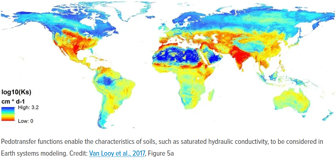
          (3) SOIL PARAMETER LAYERS: I need to have a wider selection of soil parameter options than provided by ANTS, so I have coded up a wide selection of pedotransfer functions as standard (currently, Cosby et al., Saxton & Rawls, Hodnett & Tomasella and Tóth et al. pedotransfer equation sets). I have also implemented some important automatic data checks (e.g. applying reasonable upper and lower limits to soil parameters). Base soil data for this is all taken from SoilGrids250m.

          (4) BETTER LAKES: Moving from 0.50° to 0.25° resolution and finer, many more lakes appear on the land surface. For better hydrological realism, I need these to be actually simulated but unfortunately even the SoilGrids250m layers lack soil data for many lake points. I have used gap-filling with approximate values to ensure that all lakes are included in the simulation.
     Also, large lakes: I need all lakes to be included in the land mask, but seas and oceans to be excluded (i.e. including Lake Victoria/Nnalubaale and all the US/Canadian Great Lakes, but excluding the Caspian Sea and the Black Sea). Some land-ocean masks do not follow this convention (see e.g. Lake Victoria/Nnalubaale and the Great Lakes here and also slide 6 of here, but I impose it as standard in my scripts). I am aware, unfortunately, that this approach puts me at odds with ANTS, e.g. from the ANTS documentation ATDP01
      "Lakes can be a problem in the final mask, especially with high resolution grids. Now, it may be argued that since the lakes are real they should remain in the mask to maintain reality. However, doing so may result in unacceptable noise in the lower boundary physics and the model becoming unstable and subsequently aborting ... Therefore, in most situations it is probably best to remove small lakes and only retain significant large lakes."
Although I can understand why this position is reasonable from a GCM point of view, it is extremely undesirable from a land surface point of view: for my runs I need lakes to be as correct as possible.
   *** See Extra Point 1 below ***

          (5) GLACIERS AND ICE SHEETS: For high latitude and many other applications I need a high quality land_ice layer, which makes a huge difference in many parts of the world (e.g. the Himalayas). For e.g. my MOCABORS project in Norway I needed glacier coverage and I could not see any way to use ANTS for this (the land_ice data I have seen from ANTS-generated frac ancillaries seems to be very approximate and in some cases all glaciers appear to have been simply removed as described here). To sort this out, I generated a 48 Gb raster layer at 250 m resolution composed of the union of three land_ice layers: GLIMSv6 and data on the Greenland ice sheet and Antarctica. I use this as standard in all my scripts (which again, unfortunately, puts me at odds with UK Met Office standards).

          (6) ROBUST PARAMETER AVERAGING: I need to avoid a particular hard-wired default that ANTS uses: I need my soil properties to be a calculated average of parameter values within each gridcell, rather than the dominant soil type within the gridcell (search for "The most straightforward method to aggregate" in Montzka et al. (2017) to find a short paragraph that describes the 3 main ways to do averaging of soil properties in ancillary files: it is clear from the code here that ANTS can use the dominant soil type approach only).
     There are also other issues, e.g. ANTS tries to gap-fill gridcells with no soil data "by spiral searching to the nearest adjacent land". For my runs this is undesirable because it puts in potentially erroneous soil data on many gridcells, so I prefer to leave these as no-data cells.

          (7) SOIL THERMAL PROPERTIES: I need to use equations for soil thermal properties (heat capacity and heat conductivity) that are updated from what is available in ANTS. Basically, ANTS uses equations for soil heat capacity (hcap) and soil heat conductivity (hcon) from Jones (2008) that I believe are actually completely incorrect. I have rederived these equations myself from first principles and checked the sources quoted in Jones (2008) and I now have corrected versions, but I have not yet published these myself (although they are implemented in GENHSA). Since I became aware of this situation in early 2022, I have been testing my new versions of these equations to see how much difference it makes to use them.

          (8) ROTATED AND VARIABLE-RESOLUTION GRIDS: Finally, because I use a variety of different grids in my current projects, I needed a script that could calculate ancillary files whatever my required grid resolution and extent, as well as being able to handle graticular grids (e.g. 0.25° resolution, N96 and Nxxx resolution), rotated grids (e.g. UTM, OSGB36, AMM15, UKV) and variable-resolution grids (e.g. UKCP, UKV). To be fair, I think ANTS can do all of this, but I believe it's a bit tricky (involving preparing some files 'by hand' using Iris first), but my script has been generalised and these options can be simply chosen in a straightforward menu, which means I can avoid any of these 'by hand' steps.

** A note about terminology: "regular grid" is a much-abused term and can often mean that the grid has constant resolution in terms of degrees (i.e. not variable resolution like UKCP or UKV) or that the grid is graticular (i.e. the X,Y of the grid are lines of equal longitude and latitude; the grid is unrotated) **

          (9) BETTER LAND USE (ESP. URBAN): I have replaced the urban tile of the standard frac layers I use (from IGBP/Watch ultimately) with what seems to me to be better global urban land use data from CIESIN. However, see *** Extra point 2 *** below.

          (10) PROVENANCE: Finally, the most important reason I use GENHSA rather than ANTS, however, is because using this I know exactly where all the data comes from (and can therefore justify it in a write-up). Using ANTS it still pulls in many files with rather cryptic filenames and no provenance information in the NetCDF headers, which is a significant problem. My scripts add attribute data to all NetCDF layers describing in detail where each layer comes from (and its units).

---

I want to say that, having tried to code an ancil-generator myself, it is a tough job. GENHSA has taken me several years to code up between projects at UKCEH, and has undergone a lot of refinement. This is why I can appreciate that ANTS is a very impressive system despite these points made above.

However, with the move to higher spatial resolution and a wider variety of use-needs, I believe that several of the base assumptions underlying the ANTS calculations perhaps need to be revisited and reconsidered. In a similar way that the move to convection-permitting resolutions is forcing us to revisit several climate model assumptions, I believe we must revisit some of the approximations used within the ANTS code.

I am not currently engaged with the development of ANTS, but I do have a long-term hope that some of the scripts I have coded up here can be used to improve ANTS and give it some of the functionality I feel is missing above, which I believe would make the ancillaries it creates more suitable for land surface (rather than atmospheric) simulation. My scripts are still being validated, but when that has been achieved I would be very open to the idea of working with a Python-developer in order to achieve this.

*** ANTS v1.0.0 was officially released October 2022 (see here) and I have not yet had a chance to assess it (my comments about ANTS below refer to pre-release versions up to v0.18) , so it may actually now have some of the capability below ***
​
Also note that in late 2016 a lot of documentation about the precursors of ANTS was uploaded to this ticket.

​*** Iris also needs a mention. I went through the tutorial here and my impression is that Iris is useful in a few ways (e.g. probably the easiest way to convert GRIB and PP files to NetCDF), but it doesn't replace my GENHSA script. Essentially, it loads spatial data into a 'cube' in memory (in Python) and allows you to do a lot of the same manipulations that are possible with NCO tools, with slightly less of the difficult syntax of NCO or GDAL commands. I personally have reservations about this (despite the lazy loading, I think there will be memory limitations using Iris that don't apply with NCO and GDAL), although for small grids I think it looks great. ***



Jones CP (1996). Specification of ancillary fields. Unified Model Documentation Paper 70. Please note this document states “This document has not been published. Permission to quote from it must be obtained from the Head of Numerical Modelling [at the UK Met Office]”.

Jones CP (2008). Ancillary file data sources (v.10). Unified Model Documentation Paper 70 [updated version]. Please note this document states “This document has not been published. Permission to quote from it must be obtained from the Head of Numerical Modelling [at the UK Met Office]”.

Bovis K (2012). Ancillary review - position paper. Internal position paper for the TIAN project.

Soil pedotransfer functions are an essential piece of kit for users of Land Surface Models like JULES.

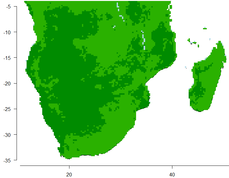
*** EXTRA POINT 1: LAKES IN HIGH RESOLUTION RUNS

I'd like to make this point here, which I believe to be an important point that will become more important as we move to higher resolution runs in the JULES Community.

Take the example of the Shire river basin in Malawi (see left). This is a fairly small river (a tributary of the Zambezi) but it has one of the world's largest lakes within its catchment (L. Malawi). How is this represented in a land surface model? Well, the current standard approach is a little (for me) odd: this lake is large enough that it goes into a separate land use type ("open water"). That sounds reasonable, but from a river modelling point of view it 'excises' the lake from the catchment: no river flow direction appears in the ancillary file over the lake area, so no river flow is calculated there. The net effect of this is that the Shire river does not start where it should start (at the river source), but actually is simulated as a much shorter river starting at the outflow point from L. Malawi.

In low resolution runs, there are very few large lakes like this, and few notice the problem (the Shire river is short and does not have any major cities on it). The River Nile does have a large lake in its headwaters (Lake Victoria/Nnalubaale) but only 7% of the flow of the Nile comes from there, therefore most of the river dynamics are arguably still well represented.

However, in high resolution runs a very large number of lakes appear (e.g. GloLakes has 27,000 lakes). Pretty much every major river system has a lake somewhere, when looked at at this resolution. If you think that, as with the Shire River above, each lake is excised from the river system it is part of, and river dynamics cannot be calculated over that missing gridcell, it's clear that this suddenly becomes a significant problem. At high resolution, many global rivers become a 'string of beads' (short reaches connecting a sequence of open lakes) and the river dynamics becomes potentially greatly fragmented.

I can see 4 possible consequences of this problem over the next few years:
     (1) LET IT HAPPEN: In each 'string of beads', the river reaches will be simulated by the river routing subroutines (TRIP or RFM), while each lake will be simulated by the Flake model. This means that the St Venant equations will greatly underestimate streamflow speeds in the reaches (each reach has hardly any water head), and there will be no flow in any of the lakes at all. I believe that this would mean that JULES will no longer be able to predict river dynamics in many global rivers.
     (2) FULL COUPLING: What would happen if we 'let it happen' and also follow a schema like UNifHy's to separate all open water from the landscape (but the rivers would remain on the land component) . While possible, for a river with many lakes, this would involve potentially several coupling locations along the river (before and after every bead of the string of beads). In addition to the problems in (1), this would involve introducing 100s of coupling locations all over all continental landmasses.

   Hydrologically speaking, all lakes are actually part of river systems (of course), so why not use a single subroutine to handle both river and lake dynamics? 
     (3) MOVE THE RIVERS INTO THE LAKE ROUTINE: We could think of river reaches as long, thin lakes and let FLake handle all of it. This would mean very few coupling points, but it would also mean that no rivers can flow anywhere, so this is not a sensible option.
     (4) MOVE THE LAKES INTO THE RIVER ROUTING: Once we have a river dynamics module that can correctly simulate overbank inundation and permanent inundation (overbank inundation has existed in JULES since 2015, but it can't currently create areas of permanent inundation), then we would no longer need an 'open water' tile in JULES at all. Following this option, FLake would become redundant as well: the river dynamics code would handle all of it.

I am flagging this problem up here because it is becoming (for me) more important as I move my work to higher resolution. At the moment, I feel the direction of travel in JULES development is towards (2), but I argue that (4) is the only long-term solution that allows rivers to be modelled as hydrologically-connected entities.

I should stress that my bespoke script does still create open water tiles (as does ANTS) and therefore does not solve this problem. It would be very straight-forward to add in a switch so that it doesn't create any lakes at all. However, without an overbank inundation module that could generate all these lakes as permanent inundation, there is little point in doing so.

*** EXTRA POINT 2: URBAN TILES THAT ARE NOT HIGH-RISE BUILDINGS

If you look closely at the urban layer ancillaries from IGBP,/Watch they seem to have hardly any cities in Asia (see e.g. image left showing the urban layer from file frac_igbp_watch_0p5deg_capUM6.6_E2OBS.nc). In terms of the state of the world in the 2020s, this seems completely wrong (see e.g. this map of global megacities).

I've not found any explanation of this in the IGBP/Watch documentation. Comparing with publicly-available distribution of global population from e.g. CIESIN, however, CIESIN seems (to me) much more in line with where global people live. What I suspect is that the term "urban" doesn't mean quite what people think it means......

I suspect that, when making maps of global urban coverage, people categorise 'urban cover' into what I could call

     urban1 = high-rise buildings (e.g. >3 stories)
     urban2 = any other populated areas (inc. towns and villages)

It seems to me that the IGBP/Watch layer is more or less urban1 as it was in ~1970 (if you compare it to e.g. this map). It seems odd to me that IGBP should have been using such an old urban layer, but I am at a loss for any other explanation: the Asian cities should definitely have been bigger even in the 2000s (the period of the Watch project).

By downloading and using CIESIN data, I have replaced the IGBP/Watch urban fractions with what is effectively urban1+urban2. This means I get the Asian cities (and forest cover in India and China immediately reduces by 50% or more in some areas), which makes me happy because it seems to me to be more realistic.

A question arises as to what JULES is actually simulating with its URBAN module: is it doing all kinds of urban cover or just urban1? If the latter, then my change here might correct urban areas but introduces an excessive amount of 'urban canyons' in tiny villages all over the world. At the moment, I don't have any solution to this: the current state of play is that I have to choose between two unsatisfactory (to me) alternatives:

     (1) Have JULES to simulate a 1970s layer of urban1 with overestimated forest cover in all areas of urban2 or
     (2) Have JULES simulate all urban areas even though I suspect it is simulating every tiny village as a (small) high-rise tile.

​Currently, my script follows alternative (2).