|
As part of the MOCABORS project 2016-21, I have been working on producing JULES simulation runs over a Norwegian domain.
I was supplied Met data for the run (with huge thanks to met.no) but the variables supplied were not the same as what the JULES model required, and ancillary files for the simulations had to be assembled from scratch. This has been accomplished through the creation of two R-based workflows (scripts) MOGEN-ANCIL.r and MOGEN-DDATA.r (see below). |
|
MOGEN-ANCIL:
I wrote an R script that generated all the ancillary files that I needed for MOCABORS and regridded them to the seNorge grid: - I have used the currently best-available global dataset for this (SoilGrids250m) and I applied Cosby's pedotransfer functions (and 3 other functions for comparison purposes) to calculate soil parameters across all of Norway (see Marthews et al. 2014). Soil parameters for each gridcell ksat (=SAT_CON in kg/m2/s), thetasat (=SM_SAT in m3/m3), soilbparam (=SOIL_B), sathh (in m of pressure head). - Land cover fractions for all PFTs as well as bare soil, urban, open water and land ice (field1391) were tricky to obtain. What I've put together for this is a temporary compromise that should perhaps be revisited in the near future: I used an old low-res 0.25deg layer for land use fractions (from IGBP), but inserted a high-res land-sea border on it and the ice element is also high-res. If you plot this layer, it looks a bit odd (a sharp and crisp coastline and glacier outlines combined with relatively chunky land use boundaries inland), but it is approximately correct and allows JULES to run. I delineated land_ice (glaciers and ice sheets) using a shapefile from the Randolph Glacier Inventory. Inland lakes I took from the null values of SoilGrids250m and the remaining land use data (frac) I took from 0.25deg eartH2Observe data (ultimately from IGBP). - I used a high resolution world coastline dataset and identified inland lake and land_ice points by their lack of data in SoilGrids. Combining that with a regridded and reformatted layer of glacier outlines from the Randolph Glacier Inventory https://www.glims.org/RGI/ , clipped to the Norwegian seNorge grid gave me high quality outlines of the Norwegian coast and glacier distribution. - Within-gridcell elevation distribution information ln(elevation-elev_min) mean and SD for each gridcell (logn_mean and logn_sd) were calculated directly from the HydroSHEDS DEM (15 arc-sec resolution) - Within-gridcell topographic index values (topographic index) mean and SD for each gridcell (topidx_mean and topidx_sd) I regridded from the 15 arc-sec topographic index values given in Marthews et al. (2015) (ultimately calculated from HydroSHEDS). |
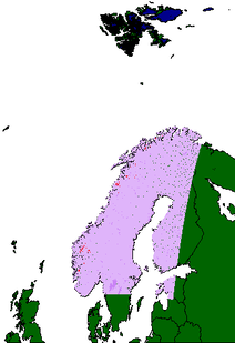
The 1km resolution MOCABORS UTM (Zone 33N) grid (violet). Lakes (purple) and glaciers (red) are shown. Green dots have no significance (they are the background showing through in a moire pattern).
MOGEN-ANCIL product variables:
This script loops through all the coordinates of the output grid and calculates all ancillary variable values at each gridcell. These include: - lsmask (1 for land, 0 elsewhere) - frac land use data is taken mostly from eartH2Observe data, but with higher-resolution land_ice and land mask data - icemask (1 for glacier or ice sheet; 0 elsewhere) - soilb (from 4 different pedotransfer functions (PTFs)) - sathh (from 4 different PTFs) - soil pH and SOC (straight from SoilGrids) - hcap and hcon - thetawilt (from 2 different PTFs) - thetacrit - thetasat (from 4 different PTFs) - soil hydraulic conductivity ksat (from 3 different PTFs) - fexp |
|
MOGEN-DDATA:
This is the element that has caused me the most problems during July-September 2021 (!). Following my own advice about obtaining driving data here, I sourced our driving data from the Norwegian Meteorological Institute (NMI). These data covered the period 2014-18, but were on a non-UTM grid (a Lambert Conformal Conic grid covering a wider extent stretching to include Jan Mayen as well) and the variables were not in a JULES-ready format. Partly because of my initial lack of familiarity with methods to transform between UTM, Lambert CC and regular long/lat coordinates, dealing with these data took some time during 2021. Eventually, I composed an R script MOGEN-DDATA.r that downloaded each day's data from the NMI's server, converted coordinates Lambert CC -> the seNorge UTM grid and then performed conversion calculations on the supplied variables (see right). Looping through all the days required, the script converts the files one-by-one, splits out the variables (JULES needs monthly data separated by variable, not daily data with all variables together) and, finally, produces 'JULES-ready' driving data. |
MOGEN-DDATA conversion calculations:
- air_pressure_at_sea_level was provided, which I could change into ambient pressure at the land surface elevation using the Barometric formula - air_temperature_2m was fine as a land surface temperature - integral_of_surface_downwelling_shortwave_flux_in_air_wrt_time was fine as shortwave downward flux. - cloud_area_fraction could be converted using the Brunt equation to get the clear-sky air emissivity and then Brutsaert's equation to calculate longwave downward flux (see Marthews et al. 2012, Theor Appl Climatol). - precipitation_amount could be converted into a rainrate (I had no information on how much precipitation is snow, so I took all to be rainfall). - relative_humidity_2m was provided, from which I could calculate specific humidity using the Goff-Gratch equation and standard assumptions about saturated vapour pressure. - and x_wind_10m & y_wind_10m I could combine into a wind speed magnitude. |
* MOGEN has nothing to do with IMOGEN, despite the similar name (and nothing to do with the Graphics Studio in South America, more's the pity!).

